What's the difference between predict_proba and decision_function in scikit-learn?
I'm studying a scikit-learn example (Classifier comparison) and got confused with predict_proba and decision_function. They plot the classification results by drawing the contours using either Z ...
stackoverflow.com
https://nittaku.tistory.com/295
14. 다중 분류 모델의 성능측정 - Performance Measure( ACU, F1 score)
캡쳐 사진 및 글작성에 대한 도움 출저 : 유튜브 - 허민석님 머신러닝을 가지고 모델을 만들어 예측하다보면, 하나의 꼬리를 가지고 여러 classifier로 만들 수 있다. 예를 들어, kNN이나 Decision Tree
nittaku.tistory.com
[모델 평가] Confusion matrix (TP, TN, FP, FN) 및 단일/다중 클래스 평가 방법 (1)
본 포스팅에서는 단일 및 다중 분류 모델에서, 모델의 성능을 평가하기 위한 다양한 performance measures 에 대하여 포스팅한다. 1. 목적 분류 모델을 평가 하기 위해서는 다양한 평가 기준들이 존
neosla.tistory.com
회귀 : 오차 평균값으로 성능 평가
분류는 복잡
분류 성능 평가 지표
정확도, 오차행렬, 정밀도(precision), 재현율 (recall), f1 score, ROC AUC
1. 정확도
모델 성능 왜곡 가능
데이터가 불균형할 수 있기 때문이다.
90개가 0이고 10개만 1일 때 모두 0으로 예측하면 정확도 90%
2. 오차행렬
| TN | FP |
| FN | TP |
이진 분류에서는 많은 데이터 중에서 중점적으로 찾아야 하는 매우 적은 수의 결괏값에 positive를 설정해 1값을 부여
예를 들어 사기 행위 예측 모델에서는 사기 행위가 positive로 1. -> 목적에 따라 설정해주자.
3. 정밀도와 재현율
정밀도 = TP / (FP+TP)
재현율 = TP / (FN+TP)
정밀도는 내 예측의 정확도 -> 분모에 P로 '예측' 한거 들어감.
재현율은 실제 값이 Positive인 대상 중에 예측과 실제 값이 1로 일치한 데이터의 비율
일치한 -> 실제로 재현한다 얼마나 실제를 잘 재현해냈느냐 -> TPR
재현율이 중요한 경우는 실제 양성인 데이터를 음성으로 잘못판단하게 되면 큰 영향이 발생하는 경우
-> 암판단 모델 / 실제 양성환자를 음성으로 잘못판단하면 사람 죽음.
정밀도가 더 중요한 경우
스팸메일 여부 -> 실제 스팸메일을 일반 메일로 분류해도 불편을 못느끼지만 실제로 음성(일반 메일)을 양성(스팸)으로 분류하면 중요 메일을 못받을 수 있음. -> FP를 줄이는데 초점
재현율, 정밀도 모두 TP를 높이는데 초점을 맞추지만
재현율은 FN , 정밀도는 FP를 낮추는데 초점을 맞추기 때문에 trade off 존재
사이킷런은 개별 데이터별로 예측 확률을 반환하는 메서드인 predict_proba()를 제공
학습이 완료된 classifier 객체에서 호출이 가능하며 X_test를 인자로 가짐
(m,n)크기로 반환 n:클래스 유형 / 첫번째는 0확률
pred_proba = lr_clf.predict_proba(X_test)
pred = lr_clf.predict(X_test)
print(pred_proba.shape)
print(pred_proba[:3])

(179, 2)
[[0.46162417 0.53837583]
 [0.87858538 0.12141462]
 [0.87723741 0.12276259]]
Binarizer 클래스 : 임계값을 설정하고 임계값보다 같거나 작으면 0으로 예측
from sklearn.preprocessing import Binarizer

custom_threshold = 0.5
pred_proba_1 = pred_proba[:,1].reshape(-1,1)

binarizer = Binarizer(threshold = custom_threshold).fit(pred_proba_1)
custom_predict = binarizer.transform(pred_proba_1)

get_clf_eval(y_test, custom_predict)


confusion matrix
[[104  14]
 [ 13  48]]
acc : 0.8491620111731844  precison : 0.7741935483870968 recall : 0.7868852459016393
임계값을 낮추면 재현율이 올라감. 정밀도는 떨어짐
왜냐하면 positive로 예측을 더 너그럽게 하기 때문에 True 값이 많아짐.
임계값을 낮춤 -> 더 많이 positive로 예측 -> TN은 작아지고 FN도 줄음 -> FP, TP가 증가
positive 예측 값이 많이 하다 보니 실제 양성을 음성으로 예측하는 횟수가 상대적으로 줄어듦(FN감소-분모가 작아짐) -> 재현율 증가
thresholds = [0.4,0.45,0.50,0.55,0.60]

def get_eval_by_threshold(y_test, pred_proba_c1, thresholds):
    for custom_threshold in thresholds:
        binarizer = Binarizer(threshold=custom_threshold).fit(pred_proba_c1)
        custom_predict = binarizer.transform(pred_proba_c1)
        print(f'임계값 : {custom_threshold}')
        get_clf_eval(y_test, custom_predict)
        print()

get_eval_by_threshold(y_test, pred_proba[:,1].reshape(-1,1), thresholds)
임계값 : 0.4
confusion matrix
[[99 19]
[10 51]]
acc : 0.8379888268156425 precison : 0.7285714285714285 recall : 0.8360655737704918
임계값 : 0.45
confusion matrix
[[103 15]
[ 12 49]]
acc : 0.8491620111731844 precison : 0.765625 recall : 0.8032786885245902
임계값 : 0.5
confusion matrix
[[104 14]
[ 13 48]]
acc : 0.8491620111731844 precison : 0.7741935483870968 recall : 0.7868852459016393
임계값 : 0.55
confusion matrix
[[109 9]
[ 15 46]]
acc : 0.8659217877094972 precison : 0.8363636363636363 recall : 0.7540983606557377
임계값 : 0.6
confusion matrix
[[112 6]
[ 16 45]]
acc : 0.8770949720670391 precison : 0.8823529411764706 recall : 0.7377049180327869
precision_recall_curve()는 예측 모델의 임곗값별 정밀도와 재현율을 반환
입력 :
y_test, 레이블 값이 1일 때의 예측 확률 값(predict_proba(X_test)[:, 1])
반환 : numpy
from sklearn.metrics import precision_recall_curve

pred_proba_class1 = lr_clf.predict_proba(X_test)[:, 1]

precisions, recalls, thresholds = precision_recall_curve(y_test, pred_proba_class1)
print(f'반환된 임계값 배열의 shape {thresholds.shape}')

thr_index = np.arange(0, thresholds.shape[0], 15)
print(f'임계값 배열의 index 10개 {thr_index}')
print(f'샘플용 10개 임계값: {np.round(thresholds[thr_index],2)}')

print(f'precision : {np.round(precisions[thr_index],2)}')
print(f'recall : {np.round(recalls[thr_index],2)}')
반환된 임계값 배열의 shape (143,)
임계값 배열의 index 10개 [ 0 15 30 45 60 75 90 105 120 135]
샘플용 10개 임계값: [0.1 0.12 0.14 0.19 0.28 0.4 0.56 0.67 0.82 0.95]
precision : [0.39 0.44 0.47 0.54 0.65 0.73 0.84 0.95 0.96 1. ]
recall : [1. 0.97 0.9 0.9 0.9 0.84 0.75 0.61 0.38 0.15]import matplotlib.pyplot as plt
import matplotlib.ticker as ticker
%matplotlib inline
def precicison_recall_curve_plot(y_test, pred_proba_c1):
precisions, recalls, thresholds = precision_recall_curve(y_test, pred_proba_c1)
plt.figure(figsize=(8,6))
threshold_boundary = thresholds.shape[0]
print(thresholds)
print(threshold_boundary)
plt.plot(thresholds, precisions[0:threshold_boundary], linestyle='-', label='precision')
plt.plot(thresholds, recalls[0:threshold_boundary], label='recalls')
start, end = plt.xlim()
plt.xticks(np.round(np.arange(start, end,0.1),2))
plt.legend()
plt.grid()
precicison_recall_curve_plot(y_test, lr_clf.predict_proba(X_test)[:, 1])
4. F1 score
정밀도 + 재현율
정밀도와 재현율이 어느 한쪽으로 치우치지 않는 수치를 나타낼때 높은 수치를 가짐.
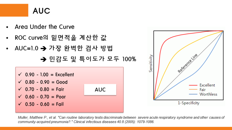
5. ROC 곡선과 AUC
이진 분류에서 중요
ROC곡선의 y좌표는 TPR (재현율)
tpr에 대응하는 지표로는 TNR(특이성) -> TN / (FP+TN)
ROC곡선의 x좌표는 FPR -> 1-TNP or FP / (FP+TN)
어떻게 FPR을 0~1까지 변경? -> 임계값 변경
FPR을 0으로 만드려면 임계값을 1로 지정 -> positive 예측 기준이 매우 높기 때문에 positive 예측 불가-> 아예 positive로 예측하지 않기 때문에 FP가 0이 되어서 Fpr은 0이됨.
FPR이 작은 상태에서 얼마나 큰 TPR을 얻을 수 있느냐가 관건
from sklearn.metrics import roc_curve

pred_proba_class1 = lr_clf.predict_proba(X_test)[:, 1]

fprs, tprs, thresholds = roc_curve(y_test, pred_proba_class1)
thr_index = np.arange(1, thresholds.shape[0],5)
print(f'임계값 배열의 index 10개 {thr_index}')
print(f'샘플용 10개 임계값: {np.round(thresholds[thr_index],2)}')

print(f'precision : {np.round(fprs[thr_index],2)}')
print(f'recall : {np.round(tprs[thr_index],2)}')
임계값 배열의 index 10개 [ 1 6 11 16 21 26 31 36 41 46 51]
샘플용 10개 임계값: [0.97 0.65 0.63 0.56 0.45 0.38 0.31 0.13 0.12 0.11 0.1 ]
precision : [0. 0.02 0.03 0.08 0.13 0.19 0.24 0.58 0.62 0.75 0.81]
recall : [0.03 0.64 0.7 0.75 0.8 0.85 0.9 0.9 0.95 0.97 1. ]
def roc_curve_plot(y_test, pred_proba_c1):
    fprs, tprs, thresholds = roc_curve(y_test, pred_proba_c1)
    plt.plot(fprs, tprs, label='ROC')
    plt.plot([0,1],[0,1], 'k--', label='Random')
    start, end = plt.xlim()
    plt.xticks(np.round(np.arange(start, end,0.1),2))
    plt.legend()
    plt.grid()

roc_curve_plot(y_test, pred_proba[:,1])

AUC는 1에 가까울수록 좋음
roc_auc_score
predict는 임계값을 변경 못하므로 Binarizer로 변환
from sklearn.preprocessing import Binarizer
binarizer = Binarizer(threshold=0.48)
pred_th_048 = binarizer.fit_transform(pred_proba[:,1].reshape(-1,1))
'머신러닝' 카테고리의 다른 글
| 파이썬 머신러닝 완벽가이드 - 4장 (0) | 2021.10.10 |
|---|---|
| 파이썬 머신러닝 완벽가이드 - 2장 (0) | 2021.09.15 |
| 파이썬 머신러닝 완벽가이드 - 1장 (0) | 2021.09.07 |
| 알고리즘 체인과 파이프라인 (0) | 2021.08.09 |
| 모델 평가와 성능 향상 (0) | 2021.08.05 |


